Normal Distribution - Simple Probabilities
A normal distribution and the empirical rule help provide us with important probability information that you must know well.
Consider a hypothetical standardized exam with a mean of 100 and a standard deviation of 20. Thus, the scores that are one, two, and three standard deviations above the mean, respectively, are 120, 140, and 160. The scores that are one, two, and three standard deviations below the mean, respectively, are 80, 60, and 40.
If we assume that the exam scores are normally distributed we know that about 68% of all data values will fall within +/- 1 standard deviation of the mean. In other words, about 68% of all of the students' scores fall between 80 and 120. This means that the probability that a randomly-selected exam score is between 80 and 120 is about 68%, or .68. This also means that the probability that a randomly-selected exam score is not between 80 and 120 is about 32%, or .32.
Let's consider this further. What's the probability of finding an exam score between 60 and 140? Since 60 and 140 are the scores that are two standard deviations from the mean, and since we know that about 95% of all data values will fall within +/- 2 standard deviations of the mean, the probability of finding an exam score between 60 and 140 is about 95%, or .95. This also means that the probability of finding an exam score that is either below 60 or above 140 will be about 5%, or .05.
Now that you have some of the fundamental probability concepts down, let's look at a few other scenarios that deal with probability and the normal distribution. We'll continue using our exam score example with mean = 100 and standard deviation = 20.
What's the probability of randomly selecting a student who scored below 100 on the exam?
We know that in any normal distribution half of the data points are above the mean and half are below. That is, the normal distribution is symmetrical. Thus the mean (100) down to zero represents exactly half, or 0.50, of the area under the entire normal curve. Since the area under the curve from the mean (100) down to zero represents 50% of the total area of the normal curve, the probability of randomly selecting a student who scored below 100 on the exam is 50%.
What's the probability of randomly selecting a student who scored above 100 on the exam? Using the same logic as that in the previous example, we see that the probability of randomly selecting a student who scored above 100 on the exam is also 50%.
What's the probability of randomly selecting a student from the 10,000 students who scored below 120 on the exam?
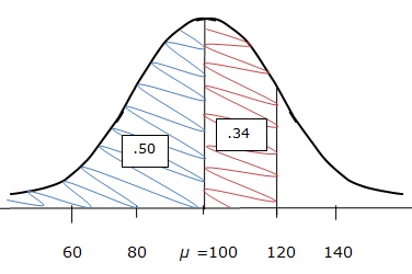
We know that a score of 120 is one standard deviation above the mean. We also know that in any normal distribution half of the data points are above the mean and half are below. Thus the mean (100) down to zero represents 0.50 of the area under the entire normal curve. We also know that about 68% of the data points will be within one standard deviation of the mean. We've already accounted for the area of the curve between the mean and zero, so let's think about what area of the curve is between one standard deviation above the mean and the mean. Since the normal curve is symmetrical and since 68% of the data points exist between one standard deviation above the mean and one standard deviation below the mean, the area between one standard deviation above the mean and the mean must be 0.34 since 0.34 is half of 0.68 (the area of the curve between one standard deviation above the mean and one standard deviation below the mean). Therefore, the probability of randomly selecting a student from the 10,000 students who scored below 120 on the exam would be 0.50 + 0.34 = 0.84 = 84%. Here is a sketch which illustrates the use of the probability facts that we have learned, applied to this problem:
Here is another example: What's the probability of randomly selecting a student who scored above 80 on the exam?
We know that a score of 80 is one standard deviation below the mean. We use logic similar to that used in the previous example, with the help of a quick sketch, to determine that the probability is 80%, or 0.80. Here is a sketch which illustrates the use of the probability facts that we have learned, applied to this problem:
As you can see, the Empirical Rule is extremely useful for determining simple probabilities for outcomes of interest for normally-distributed data.
Consider a hypothetical standardized exam with a mean of 100 and a standard deviation of 20. Thus, the scores that are one, two, and three standard deviations above the mean, respectively, are 120, 140, and 160. The scores that are one, two, and three standard deviations below the mean, respectively, are 80, 60, and 40.
If we assume that the exam scores are normally distributed we know that about 68% of all data values will fall within +/- 1 standard deviation of the mean. In other words, about 68% of all of the students' scores fall between 80 and 120. This means that the probability that a randomly-selected exam score is between 80 and 120 is about 68%, or .68. This also means that the probability that a randomly-selected exam score is not between 80 and 120 is about 32%, or .32.
Let's consider this further. What's the probability of finding an exam score between 60 and 140? Since 60 and 140 are the scores that are two standard deviations from the mean, and since we know that about 95% of all data values will fall within +/- 2 standard deviations of the mean, the probability of finding an exam score between 60 and 140 is about 95%, or .95. This also means that the probability of finding an exam score that is either below 60 or above 140 will be about 5%, or .05.
Now that you have some of the fundamental probability concepts down, let's look at a few other scenarios that deal with probability and the normal distribution. We'll continue using our exam score example with mean = 100 and standard deviation = 20.
What's the probability of randomly selecting a student who scored below 100 on the exam?
We know that in any normal distribution half of the data points are above the mean and half are below. That is, the normal distribution is symmetrical. Thus the mean (100) down to zero represents exactly half, or 0.50, of the area under the entire normal curve. Since the area under the curve from the mean (100) down to zero represents 50% of the total area of the normal curve, the probability of randomly selecting a student who scored below 100 on the exam is 50%.
What's the probability of randomly selecting a student who scored above 100 on the exam? Using the same logic as that in the previous example, we see that the probability of randomly selecting a student who scored above 100 on the exam is also 50%.
What's the probability of randomly selecting a student from the 10,000 students who scored below 120 on the exam?
We know that a score of 120 is one standard deviation above the mean. We also know that in any normal distribution half of the data points are above the mean and half are below. Thus the mean (100) down to zero represents 0.50 of the area under the entire normal curve. We also know that about 68% of the data points will be within one standard deviation of the mean. We've already accounted for the area of the curve between the mean and zero, so let's think about what area of the curve is between one standard deviation above the mean and the mean. Since the normal curve is symmetrical and since 68% of the data points exist between one standard deviation above the mean and one standard deviation below the mean, the area between one standard deviation above the mean and the mean must be 0.34 since 0.34 is half of 0.68 (the area of the curve between one standard deviation above the mean and one standard deviation below the mean). Therefore, the probability of randomly selecting a student from the 10,000 students who scored below 120 on the exam would be 0.50 + 0.34 = 0.84 = 84%. Here is a sketch which illustrates the use of the probability facts that we have learned, applied to this problem:
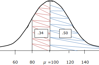
Here is another example: What's the probability of randomly selecting a student who scored above 80 on the exam?
We know that a score of 80 is one standard deviation below the mean. We use logic similar to that used in the previous example, with the help of a quick sketch, to determine that the probability is 80%, or 0.80. Here is a sketch which illustrates the use of the probability facts that we have learned, applied to this problem:
As you can see, the Empirical Rule is extremely useful for determining simple probabilities for outcomes of interest for normally-distributed data.
|
Related Links: Math Probability and Statistics Shapes of Distributions Frequency Table - Categorical Data |
To link to this Normal Distribution - Simple Probabilities page, copy the following code to your site: